With the following material we want to provide the reader of the paper with some additional information on our work. See the supporting material to read more about the formulas and model parameters and a detailed description of the extension to the global SLIR model. Headlines and enumerations correspond to sections in the main article.

In the following we present animated gif-files visualizing our simulation results. In order to achieve outcomes that are better visible in the graphical representation, we multiplied the basic reproduction number ρ and hence the transmission rate α by 1.25 in comparison to the one used in the paper. Click on the pictures in order to start the animations.

Representation via Time Series

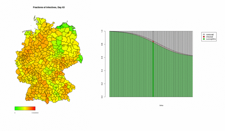
In the following three examples, the numbers of initially infected individuals correspond to week 5/2005 in the dataset, multiplied by 500 in order to speed up the process; the simulations show the development over the next 120 days. This first animation displays two graphical representations of the spread of a disease: On the left, a map of Germany coloured in accordance to the degree of affection, indicating the spatial spread of the epidemic at each instant of time. On the right, a time series showing the average fractions of susceptible (green), infected (red), and recovered (white) individuals all over Germany.

Fractions of Infectives and Sizes of the Epidemic

Next, we want to display side-by-side the proportion of infectious individuals and the size of the epidemic in each district, where the latter is defined as the fraction of individuals of the total population that have been affected by the disease (in the current epidemic) until the considered instant of time. Note that the two maps use different scales since the size of the epidemic is certainly larger than the infected fraction.

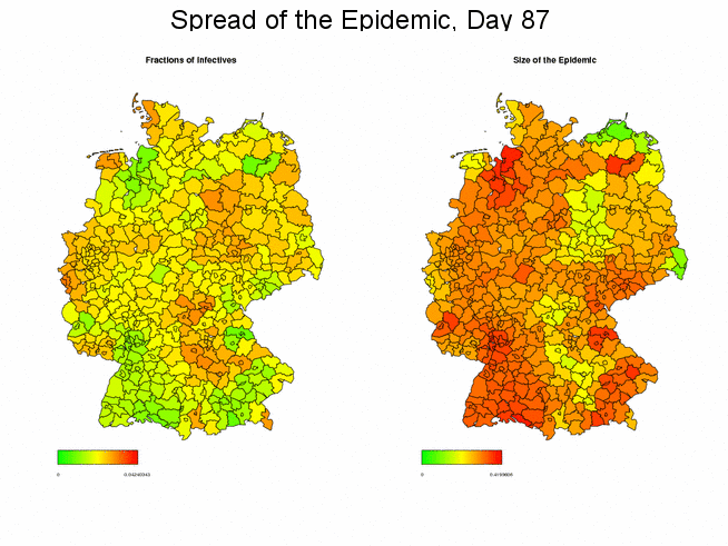
The average final size of the simulated epidemic—i.e. the size of the epidemic when it is over—reads 0.385. The average fraction of individuals not having been affected by the disease hence reads 0.615. Plugging in this value into formula (9) from the paper, we obtain that the reproduction number ρ used for the simulations must have been about 1.26, which proves true.

Stochastic vs. Deterministic Global SIR Model

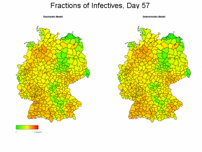
The following figure compares the deterministic with one stochastic simulation of the spread of a disease. Both applications generally yield the same course and magnitude of the spread, though certainly declining in some districts.

Impact of the Connectivity Matrix

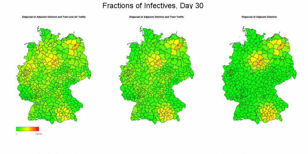
In the next two animations, we examine the effect of the connectivity matrix γ on the (deterministic) simulation outcomes by once taking into account the full connectivity matrix (i.e. dispersal between adjacent regions and train and air traffic), once ignoring the air traffic, and once restricting the mixing to only the migration between adjacent regions. In the first simulation, we again use week 5/2005 from the dataset as starting situation. The results show that the epidemic spreads rather uniformly through Germany in case of full migration network, and more concentratedly otherwise, but when reaching the end of the epidemic, the final sizes will be the same in all three scenarios.

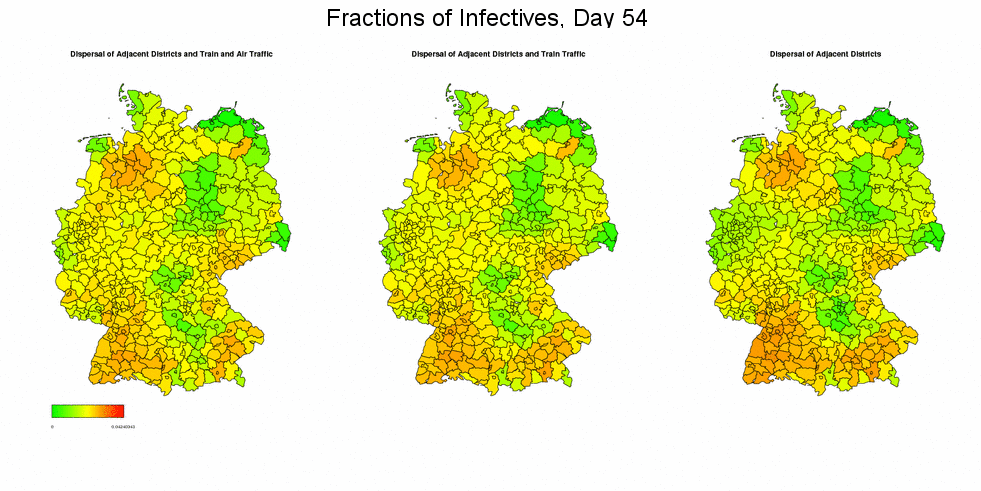
These effects becomes clearer when concentrating the initial infectives in few regions: In the following simulation we chose the districts Munich in the South (population density 3955, included in the train and air network model), Braunschweig in the North (population density 1278, included in the train but not in the air network model), and Müritz in the East (population density 41, neither included in the train nor air network model) as sources of the epidemic by setting their fractions of infectives equal to 0.5 while leaving all other districts unaffected. (For better visibility, the maps in the now following graphics display the square roots of the actually simulated data. Presentations start at day 10.)

Simulating with Different Resolutions

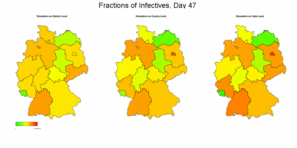
Next, we run the deterministic simulation of the spread of an epidemic, initialized with the data from week 6/2005 (times 500), on district, county, and state level. In all three cases we present the resulting fractions of infective individuals on state level. Edge effects, as they were already mentioned in the paper, have certainly deeper impact when simulating on a coarser level, concerning the overall fractions of infectives in Germany.